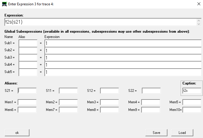
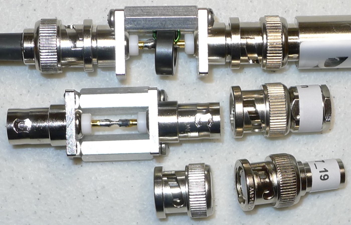
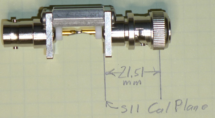
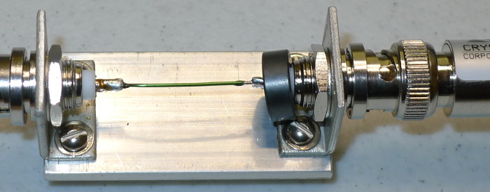
S21 Adapter
|
One Inch Spacing using Aluminum Bar Stock
|
One Inch Spacing using Aluminum Bar Stock
|
Comparison With
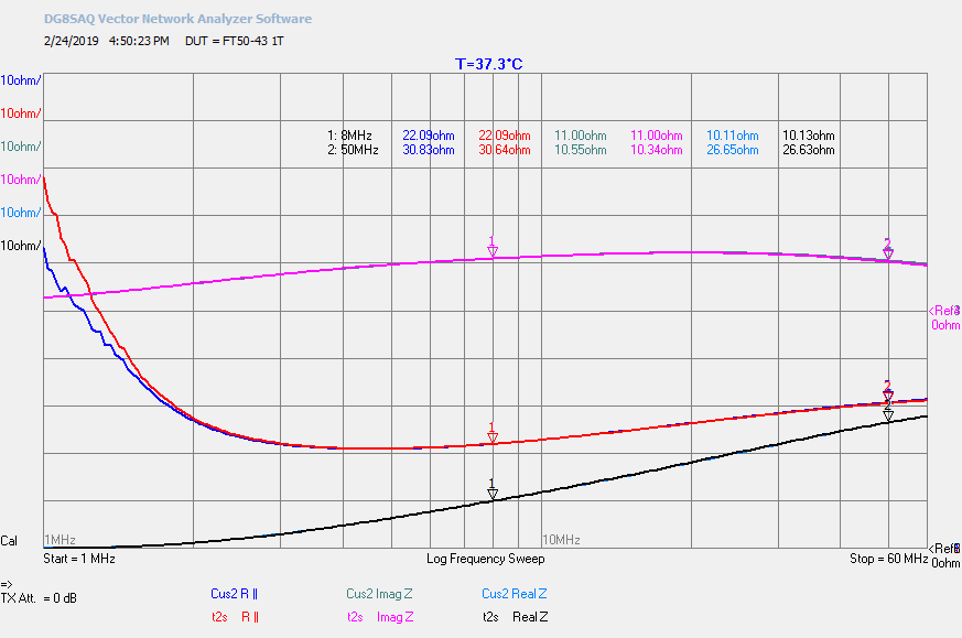
Applying and Measuring Ferrite Beads, Part III ~ Measurements
Page 7, Figure 8
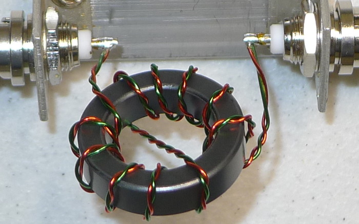
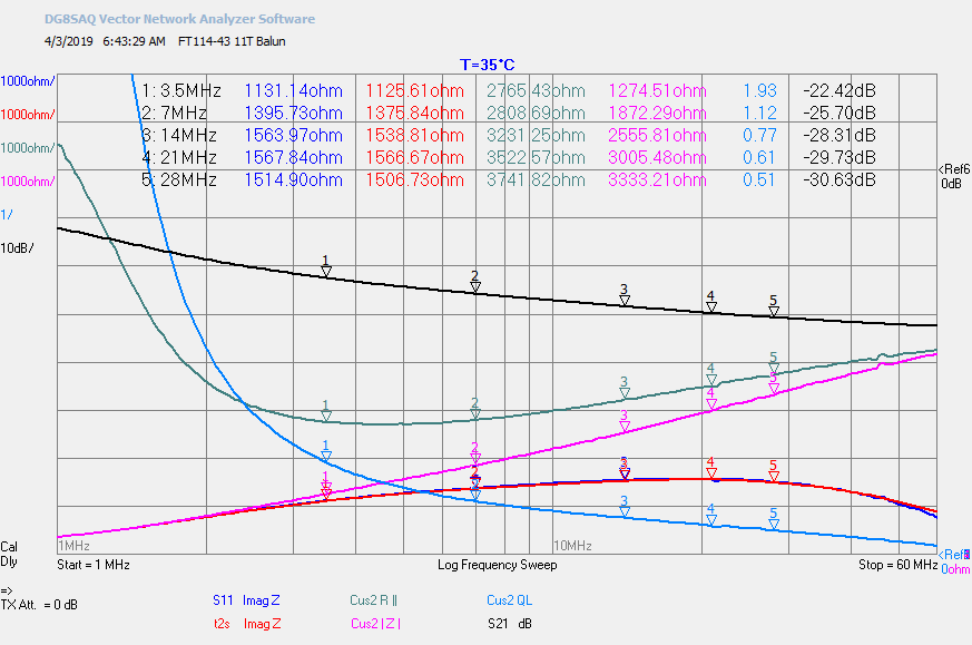
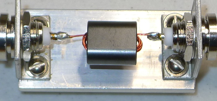
FT114-43 11T 2x#22 Balun
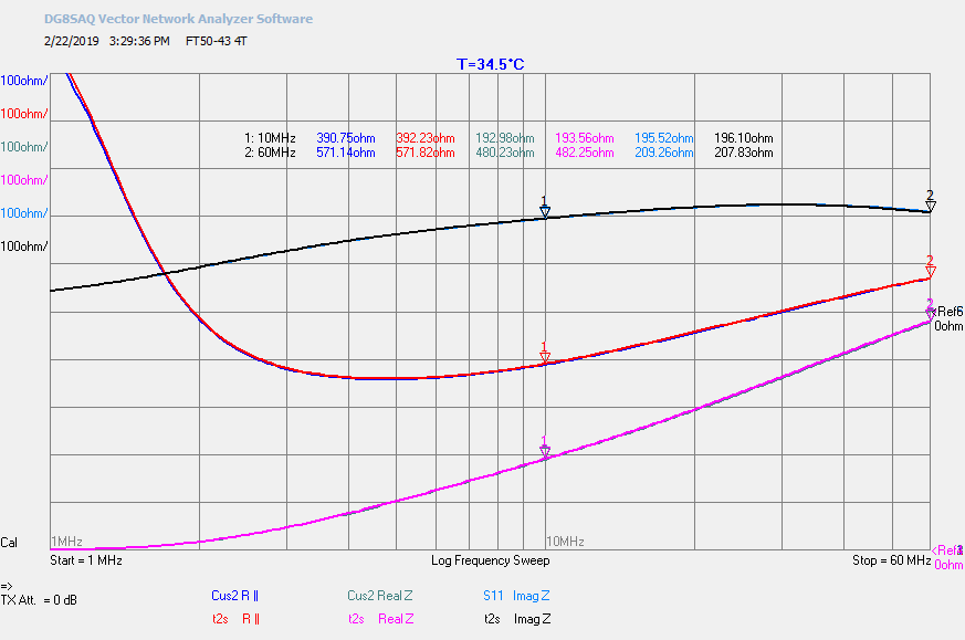
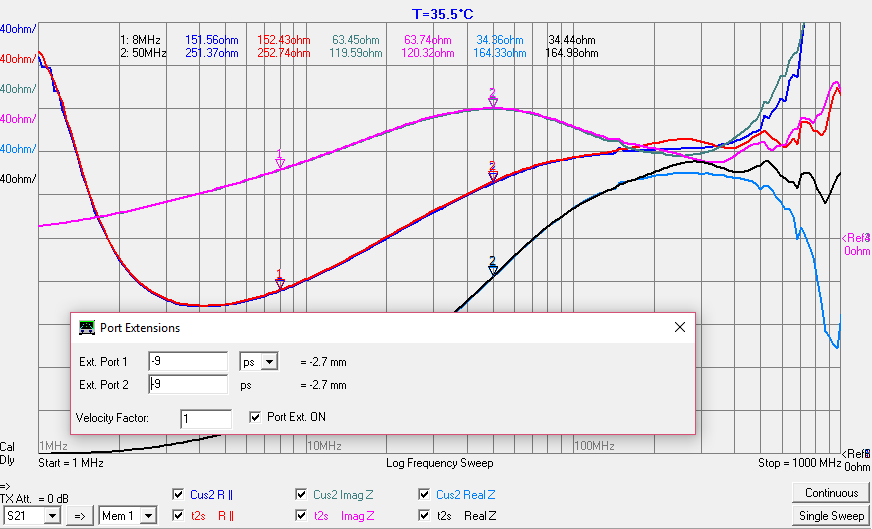
Port Extension set for (S11 ImagZ == t2s ImagZ) = 10ps
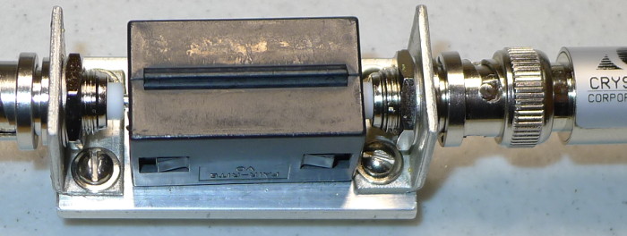
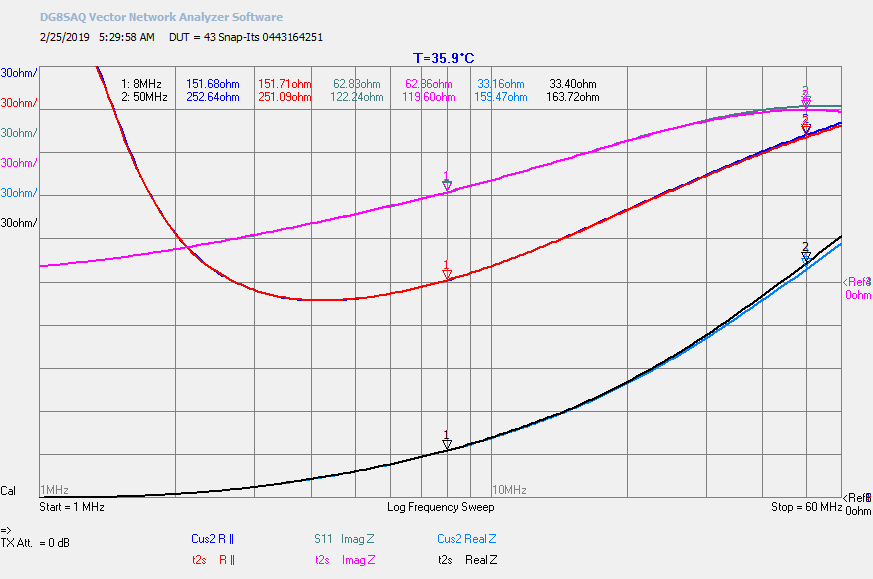
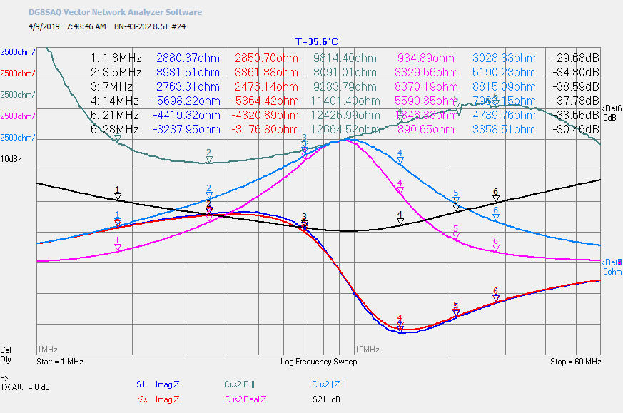
BN-43-202 8.5T #24
Port Extension set for (S11 ImagZ == t2s ImagZ == 0) = -8ps
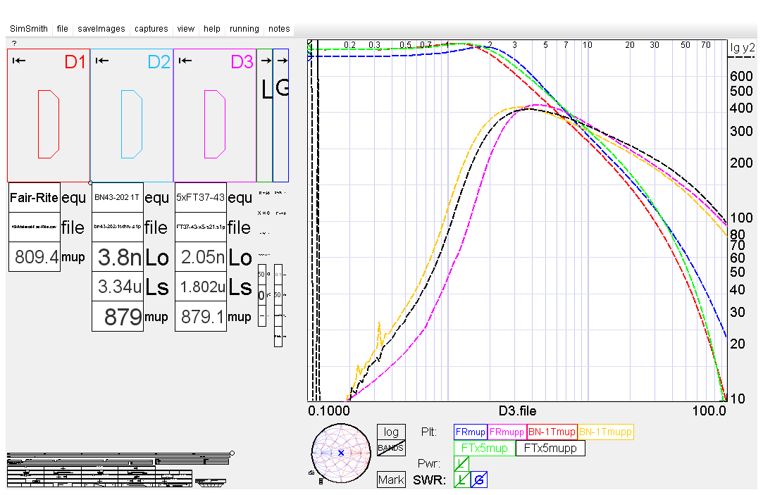
Measuring and Plotting 43 Ferrite Complex Permeability using SimSmith
Measuring 31 Material
Measuring 43 Material
Measuring 52 Material
Measuring 61 Material
Measuring 67 Material
|
| D1 Text | D2 Text | D Text using μ = μ' - jμ" |
|---|---|---|
//Fair-Rite
$data=file[]; // Fair-Rite File
mup = $data.R;
$mupp = $data.X;

Plot("F-Rmup",mup,y2);
Plot("F-Rmupp",$mupp,y2);
|
//BN43-202 1T
$data=file[];  // S11 File
Lo;
$Rs = $data.R;
$Xs = $data.X;
Ls = $Xs/(2*Pi * G.MHz * 1M);
mup = Ls / Lo;
$Q = $Xs / $Rs;
$upp = mup / $Q;

Plot("BN1Tmup",mup,y2);
Plot("BN1Tmupp",$upp,y2);
|
//BN43-202 1T Using u'-ju"
$data=file[];  // S11 File
Lo;
$mu = -j * $data / (2*Pi * G.MHz * 1M * Lo);
Plot("mup",$mu.R,y2);
Plot("mupp",-$mu.I,y2);
|
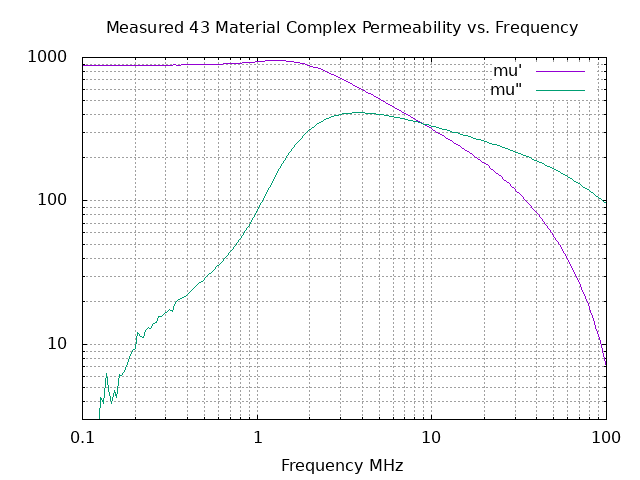
Plotting FT37-43 x 5 Complex Permeability using gnuplot
| gnuplot File Text |
|---|
set terminal png
set output 'gp-cp.png'
set datafile commentschars "!#" # s1p File comment compatible
set grid xtics ytics
set grid mxtics mytics
set key top right
set xlabel "Frequency MHz"
set title "Measured 43 Material Complex Permeability vs. Frequency"
set yrange [3:1000]
set logscale xy

Lo = 2.05e-9 # Permeability=1 Inductance
i = {0,1}
Zs(a,b) = 50 * (1 + (a+b*i))/(1 - (a+b*i)) # s1p MHz S RI R 50 to Zs
Rs(a,b) = real(Zs(a,b))
Xs(a,b) = imag(Zs(a,b))
Ls(f,a,b) = Xs(a,b)/(2*pi * f * 1e6)
mup(f,a,b) = Ls(f,a,b) / Lo
Q(a,b) = Xs(a,b) / Rs(a,b)
mupp(f,a,b) = mup(f,a,b) / Q(a,b)

plot \
'FT37-43-x5-s21.s1p' using ($1):(mup($1,$2,$3)) with lines title "mu'", \
'FT37-43-x5-s21.s1p' using ($1):(mupp($1,$2,$3)) with lines title "mu\""
|
| gnuplot File Text, Solving for μ = μ' - jμ" |
|---|
set terminal png
set output 'gp-cp.png'
set datafile commentschars "!#" # s1p File comment compatible
set grid xtics ytics
set grid mxtics mytics
set key top right
set xlabel "Frequency MHz"
set title "Measured 43 Material Complex Permeability vs. Frequency"
set yrange [3:1000]
set logscale xy

Lo = 2.05e-9 # Permeability=1 Inductance
i = {0,1}
Zs(a,b) = 50 * (1 + (a+b*i))/(1 - (a+b*i)) # s1p MHz S RI R 50 to Zs
mu(f,a,b) =  -i * Zs(a,b) / (2 * pi * f * 1e6 * Lo) # mu() = u' - u"
plot \
'FT37-43-x5-s21.s1p' using ($1):(real(mu($1,$2,$3))) with lines title "mu'", \
'FT37-43-x5-s21.s1p' using ($1):(-imag(mu($1,$2,$3))) with lines title "mu\""
|
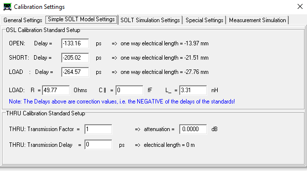
Example Calibration Settings
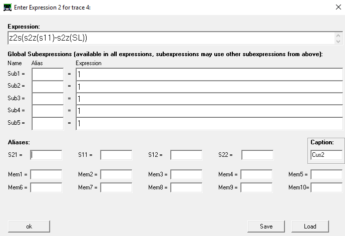
Cus2 Window
Cus3 Window