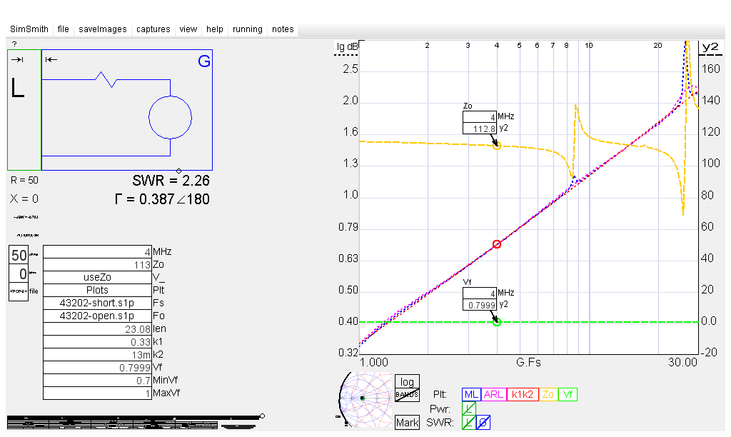
| Using SimSmith for Transmission Line (TL) open circuit and short circuit condition evaluation of TL nominal impedance Zo, and Zo Loss, matched loss, and k1 k2 loss per 100 feet, Impedance, and Velocity Factor. |
SimSmith Window
| SS G Block | Notes |
|---|---|
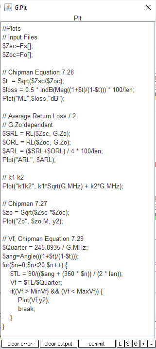
| G.Plt | Edit Plt using cut and paste text below.
Or load SSTLeval.zip |
| G.Fs | Short condition measurement file, 43202-short.s1p for this example. (File link below) |
| G.Fo | Open condition measurement file, 43202-open.s1p for this example. (File link below) |
| G.len | TL length in feet |
| G.k1 | Adjust k1 for k1k2 Loss Trace match at low frequency. 0.33 in this example. |
| G.k2 | Adjust k2 for high frequency k1k2 Loss Trace match, may need minor k1 adjustments. 0.013 in this example. |
| G.Vf | Computed Velocity Factor |
| G.MinVF G.MaxVF | Set to expected Velocity Factor range |
| Plot Trace | Description |
| ML | Matched Loss using
"Theory and Problems of Transmission Lines"
by Robert A. Chipman, Page 135 Equation 7.28
Set SimSmith G.len to TL length for per 100' computations. |
| ARL | Average of Return Loss, in dB, divided by two, for one way loss.
Adjust SimSmith G.Zo for match to Loss Trace. TL Zo = 113Ω in this example. AKA: Transmission Line Insertion Loss with Load and Generator Impedance equal to Transmission Line Nominal Impedance. |
| k1k2 | Computed loss using k1, copper loss, and k2, dielectric loss. |
| k0 loss term using copper wire AWG charts
#18 DCr = 6.385Ω/1000' = 1.277Ω/200' k0 = 20 * Log10((113 + 1.277/2) / 113) = 0.0489 | |
| Zo | Zo using "Theory and Problems of Transmission Lines" by Robert A. Chipman, Page 134 Equation 7.27 |
| Vf | Velocity factor using Chipman Equation 7.29 |
| SimSmith G.Plt Window | SimSmith G.Plt Text |
|---|---|
|
//Plots
// Input Files
$Zsc=Fs[];
$Zoc=Fo[];

// Chipman Equation 7.28
$t  = Sqrt($Zsc/$Zoc);
$loss = 0.5 * IndB(Mag((1+$t)/(1-$t))) * 100/len;
Plot("ML",$loss,"dB");

// Average Return Loss / 2
// G.Zo dependent
$SRL = RL($Zsc, G.Zo);
$ORL = RL($Zoc, G.Zo);
$ARL = ($SRL+$ORL) / 4 * 100/len;
Plot("ARL", $ARL);

// k1 k2
Plot("k1k2", k1*Sqrt(G.MHz) + k2*G.MHz);

// Chipman 7.27
$zo = Sqrt($Zsc *$Zoc);
Plot("Zo", $zo.M, y2);

// Vf, Chipman Equation 7.29
$Quarter = 245.8935 / G.MHz;
$ang=Angle(((1+$t)/(1-$t)));
for($n=0;$n<20;$n++) {
    $TL = 90/(($ang + (360 * $n)) / (2 * len));
    Vf = $TL/$Quarter;
    if((Vf > MinVf) && (Vf < MaxVf)) {
        Plot(Vf,y2);
        break;
    }
}
|
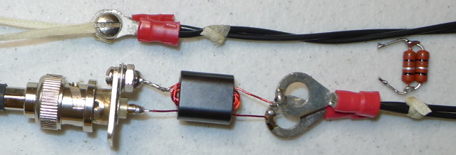
Example Balun and Transmission Line
|
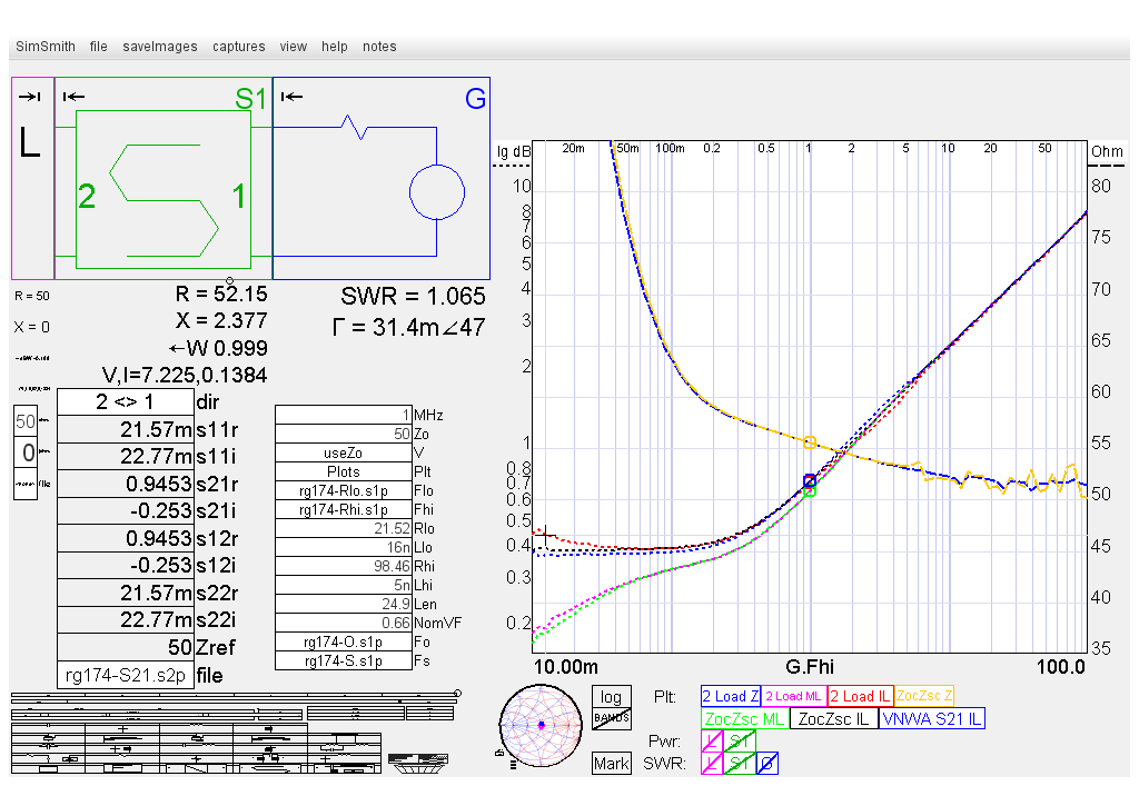
Two Load Method, Zlor/Zhir
|
James E. McKay, Electronic Design, November 1976
Albert E. Weller, WD8KBW, QEX, Nov/Dec 2001 Two Load Method SimSmith port by Dan Maguire, AC6LA |
Type RG174, solid conductor, Example
Files RG174-80p.zip
| G.Plt Input | Description |
|---|---|
| Flo | S11 Rlo file |
| Fhi | S11 Rhi file |
| Rlo | Measured low resistance load |
| Llo | Low Load inductance, adjust for smooth 2 Load Z trace |
| Rhi | Measured high resistance load |
| Lhi | High Load inductance, adjust for smooth 2 Load Z trace |
| Len | TL length |
| NomVF | Nominal TL VF. (not critical) |
| Fo | S11 Open Condition file |
| Fs | S11 Short Condition file |
| Trace | Description |
| 2 Load Z | Two Load Method Impedance |
| 2 Load ML | Two Load Method Matched Loss |
| 2 Load IL | Insertion Loss at G.Zo using Return Loss average
ZocZsc from Two Load ML using SimSmith T() function |
| ZocZsc Z | Chipman Equation 7.27 |
| ZocZsc ML | Chipman Equation 7.28 |
| ZocZsc IL | Insertion Loss at G.Zo using Return Loss average |
| VNWA S21 IL | Measured S21 Insertion Loss |
| G.Plt Text |
|---|
//Plots
$Zlo=Flo[];
$Zhi=Fhi[];
Rlo;Llo;Rhi;Lhi;
$Xlo =2*Pi * G.MHz * 1M * Llo;
$Llo = Rlo + j*$Xlo;
$Xhi = 2*Pi * G.MHz * 1M * Lhi;
$Lhi = Rhi + j*$Xhi;
$Zo = Sqrt(
  (($Zlo-$Llo)*$Lhi*$Zhi - ($Zhi-$Lhi)*$Llo*$Zlo)  /
  ($Zlo-$Zhi-$Llo+$Lhi)   );
Plot("2 Load Z",$Zo.M,"Ohm",y2);

$gL = Atanh($Zo * ($Lhi - $Zhi) / (($Lhi * $Zhi) - $Zo^2));
$Neper = 20/Ln(10);
$ML = Real($gL) * $Neper / Len * 100;
Plot("2 Load ML",$ML,"dB");

$Zoc = T(1P, Len, $Zo, NomVF, $ML);
$Zsc = T(1f, Len, $Zo, NomVF, $ML);
$RLoc = RL($Zoc, G.Zo);
$RLsc = RL($Zsc, G.Zo);
$IL = ($RLoc + $RLsc) / 4 / Len * 100;
Plot("2 Load IL",$IL);

$Zoc=Fo[];
$Zsc=Fs[];
$Zo = Sqrt($Zoc * $Zsc);
Plot("ZocZsc Z",$Zo.M,y2);

$t = Sqrt($Zoc/$Zsc);
$ML = 0.5 * IndB(Mag((1+$t)/(1-$t))) * 100/Len;
Plot("ZocZsc ML",$ML);

$RLoc = RL($Zoc, G.Zo);
$RLsc = RL($Zsc, G.Zo);
$IL = ($RLoc + $RLsc) / 4 / Len * 100;
Plot("ZocZsc IL",$IL);

Plot("VNWA S21 IL",-10*Log10(L.P)*100/Len);
|